GPlates Web Service
A couple of packages already exist for using GPlates reconstructions to create palaeogeographical maps in R:
- NonaR/paleoMap (https://github.com/sonjaleo/paleoMap)
- LunaSare/gplatesr (https://github.com/LunaSare/gplatesr)
Both of these download from GPlates Web Service (GWS). I’ve borrowed some of their functions for this lab group.
If you’re unfamiliar with RStudio or RMarkdown (.Rmd files), then the code sections are placed in ‘chunks’ like the one below. You can run individual lines by ⌘ + Enter or Ctrl + Enter, or run the whole chunk using the little green arrow to the top right of each chunk. Try with this chunk below if you want.
library(broom)
library(dplyr)
library(forcats)
library(ggplot2)
library(ggthemes)
library(mapproj)
library(purrr)
library(readr)
library(rgdal)
library(stringr)
library(tibble)
# library(tidyverse) # a quick way to load packages, but slow for Binder.

list.files("functions/", pattern = "\\.R", full.names = TRUE) %>%
    walk(source)
Not all of the chunks should be run on Binder as some of the code will take a long time or fail to execute.
Downloading from GWS
GWS can reconstruct the locations of points, coastlines, plates, paths, and features back into the past (https://github.com/GPlates/gplates_web_service_doc/wiki). It can also use a variety of different reconstructions. Most relevant is perhaps the Golonka (2007) model, which is often used for palaeocoordinate reconstruction in the Palaeobiology Database (PBDB).
The process is:
- Download outlines of the continental coastlines.
- Download outlines of the tectonic plates.
- Read and convert these into a format that R and ggplot2 can use,
- this uses the packages rgdal, readr, and broom.
- Plot,
- in this case with ggplot.
Do not run this code on Binder. The code below does these steps by downloading the data, which will likely take some time.
coastline_gws_url <-
  "http://gws.gplates.org/reconstruct/coastlines/?time=155&model=GOLONKA"
polygons_gws_url <-
  "http://gws.gplates.org/reconstruct/static_polygons/?time=155&model=GOLONKA"

kimmeridgian_coastlines <-
  rgdal::readOGR(coastline_gws_url) %>%
    broom::tidy()
kimmeridgian_polygons <-
  rgdal::readOGR(polygons_gws_url) %>%
    broom::tidy()
This chunk below replicates the above using data I’ve already downloaded from GWS and stored in the GitHub repository, and can be used on Binder. It has the same steps of loading and tidying the data, then includes the commands to plot with ggplot2.
Feel free to run this code on Binder.
# Load and tidy the data
kimmeridgian_coastlines <-
  readOGR(
    "data/GWS/Matthews_etal_GPG_2016_Coastlines_reconstructed_155.00Ma.gmt"
  ) %>%
    tidy()
kimmeridgian_polygons <-
  readOGR(
    "data/GWS/Matthews_etal_GPG_2016_Polygons_reconstructed_155.00Ma.gmt"
  ) %>%
    tidy()

ggplot() +
  geom_map(
    data = kimmeridgian_polygons,
    map = kimmeridgian_polygons,
    aes(x = long, y = lat, map_id = id),
    fill = "#D8D8D8"
  ) +
  geom_map(
    data = kimmeridgian_coastlines,
    map = kimmeridgian_coastlines,
    aes(x = long, y = lat, map_id = id),
    colour = "#222222", fill = NA, size = 0.3
  ) +
  coord_map("mollweide") +
  map_border() +
  theme_map()
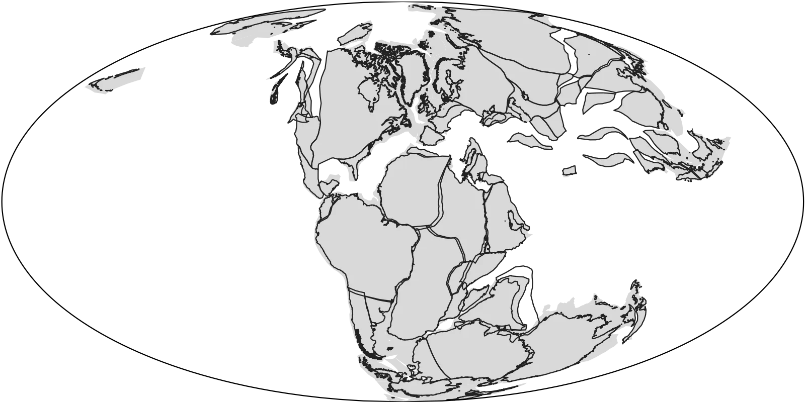
When plotting, the data are added as layers, each plotting over the other: plate polygons at the bottom then coastlines on top. I’ve also set the map projection to be Mollweide, but you can play with this and change it to others included in the mapproj package function mapproject. Options include "Gilbert", "fisheye", and "hex". (Use, for example, coord_map("fisheye", n = 0.7) to add extra arguments.)
Additionally I’ve added a border (map_border(), in the functions folder) and used a basic theme (theme_map()) to get a plain background.
How R plots these map data
The positions and extent of map areas from data in GPlates are stored as a series of polygons. Each region is outlined by a series of points that form a closed shape, filled with a particular colour. This is exported from GPlates as OGR-GMT format, with file extension .gmt, which lists each point that marks the corner of a polygon. In R, broom converts this to a tibble (similar to a data.frame) that has the x and y locations of each point, and a series of columns that identify which polygon that point belongs to. These ID columns are important to make sure that polygons contain the correct points and are closed properly. Without these, there would only be a single shape that would stretch across the whole globe and not make much sense.
Not quite right
GWS is convenient for data and access, but the results in the plot above show the current continental coastlines and the plates. This does not reflect the ancient coastlines that we’re really after. Also, many of the countries are cross-cut by the polygons that form the sections in the model, which are untidy and typically not visible.
We need to go to the next level: true palaeogeographical reconstructions. Fortunately GPlates offers that too.
Exercises 2
- Have a look at the GWS documentation. What address would you use to get reconstructed coastlines in the early Carboniferous using the Matthews et al. (2016) model?
- Open an example of the OGR-GMT data from the GWS, either from the
data/GWSfolder or by downloading it. Can you see how the polygons are stored? How are different polygons identified? - Now look at the tidied version in R, i.e.\
kimmeridgian_coastlinesorkimmeridgian_polygons. By default this will only show the first 10 rows, but you can see more with, for example,head(kimmeridgian_polygons, n = 50L). Can you see how the OGR-GMT data is transferred to this tidy format? - Play around with the inputs to the plot above. How messy or colourful can you make this map? What options are there in
theme_map()? (Hint: use?theme_mapto see.)
References
Cao, W., Zahirovic, S., Flament, N., Williams, S., Golonka, J. and Müller, R.D. 2017. Improving global paleogeography since the late Paleozoic using paleobiology. Biogeosciences 14 (23): 5425–5439. doi:10.5194/bg-14-5425-2017
Golonka, J. 2007. Phanerozoic paleoenvironment and paleolithofacies maps: Mesozoic. Geologia 33 (2): 211–264.
Matthews, K.J., Maloney, K.T., Zahirovic, S., Williams, S.E., Seton, M. and Müller, R.D. 2016. Global plate boundary evolution and kinematics since the late Paleozoic. Global and Planetary Change 146: 226–250. doi:10.1016/j.gloplacha.2016.10.002
Leave a comment