Adding Fossil Occurrence Data

Now that you’ve spent lots of time making a pretty map, let’s plot some fossils on top of it.

Of course, being me and having used Jurassic data, we’re going to plot some ichthyosaurs. In this instance, the occurrence data comes from the PBDB, downloading ichthyosaur occurrences with these filters:

• Callovian–Tithonian (166-145 Ma)
• all levels of taxonomy – no filtering.

The PBDB has its own web API (https://paleobiodb.org/data1.2) from which you can get occurrences, collections, taxonomy and other things. In the code chunk below I’ve crafted the URL to download the data, but this is already in the repo so doesn’t need to be run.

Do not run the following chunk on Binder, the data are already in the repo.

#### DO NOT RUN THIS CHUNK ####
pbdb_url <-
  "https://paleobiodb.org/data1.2/occs/list.csv?base_name=Ichthyosauromorpha&interval=Callovian,Oxfordian,Kimmeridgian,Tithonian&show=paleoloc"

occ_ichthyosaurs <-
  read_csv(pbdb_url)

The part of the URL show=paleoloc is the important bit as the PBDB has already computed the palaeocoordinates of most occurrences using their modern location and the ages of the occurrences. Conveniently using the same default GPlates model as the palaeogeography.

Adding Occurrence Points

With that all done, use the chunk below to add the occurrences onto the base map. These are plotted with geom_point(), which you may be familiar with, setting the x and y values to the palaeolongitude and palaeolatitude respectively.

You can run this chunk and the following ones.

occ_ichthyosaurs <-
  read_csv("data/occurrences/2021-02-18-ichthyosaur-occurrences.csv")
occ_plot <-
  map_plot +
    geom_point(
      data = occ_ichthyosaurs,
      aes(
        x = paleolng,
        y = paleolat
      )
    )
occ_plot

Occurrences of ichthyosaurs from the Callovian–Tithonian. Palaeogeographical map shows the distribution of land in the Kimmeridgian (155 Ma) reconstructed by Cao et al. (2017). Occurrences of Ichthyosauromorpha are from the Palaeobiology Database.

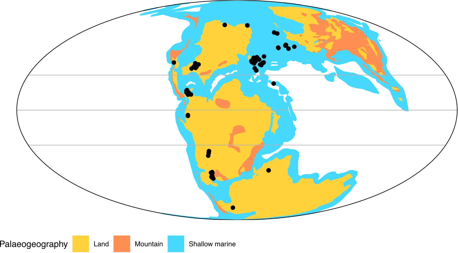
Mismatch in Locations

The more eagle-eyed of you may notice that some of these marine ichthyosaur occurrences are located resolutely in the middle of landmasses. There are a few possible reasons for that:

1. The palaeogeographical reconstruction is wrong.
2. The modern location for the occurrence is wrong, so the palaeocoordinates are wrong.
3. The age of the occurrence is wrong, so its reconstructed position is wrong.

These three are worth considering further.

Incorrect palaeogeographical reconstruction is perhaps the most obvious answer: these reconstructions are difficult and there will always be some uncertainty with reconstructing the earth 155 million years ago. However, the method of Cao et al. (2017) included palaeoenvironments reconstructed using PBDB data to improve confidence in the borders of sea and land. The palaeogeography should match the PBDB well then, particularly in well-studied and sampled periods and locations. There are, however, some parts that cannot certainly reconstructed because of a lack of data, rock availability, or accessibility.

Incorrect modern location may be the easiest to discount as localities tend to be spatially constrained and identifiable, even in older literature. This being the case, there should only be minor error in the locations of occurrences (~10s km).

Incorrect age assignment is probably the most likely cause, or perhaps better imprecise ages. The palaeocoordinates calculated for each occurrence in the PBDB use the midpoint of its temporal range. Sometimes this range can be quite large, such as the several species of Undorosaurus that cover the whole Late Jurassic (163.5–145 Ma in GTS 2020/03). Those specimens from Patagonia that are plotted in the middle of the land are also similarly imprecisely dated. Their palaeocoordinates are reconstructed to the middle Kimmeridgian, whereas they are likely later (given the occurrence of ichthyosaurs from similar locations) when there was a sea there to swim in.

As the ichthyosaur occurrences included cover over 20 Ma of earth history there will be changes in palaeogeography, and some potentially imprecise dating.

The ways around this are to have more time slices with the occurrences plotted, but this complicates the code and any plots, and such precise reconstructions may not be available. Alternatively, aim to use only the most precisely dated occurrences, if possible, but this can remove lots of useful data. Ultimately, you may just have to accept that some marine occurrences may appear on land, or vice versa.

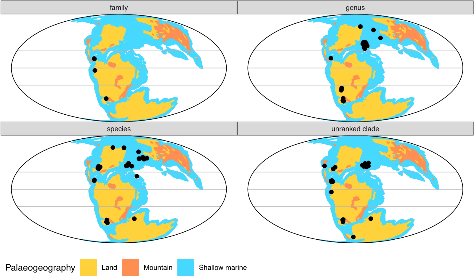
Going Further 2: Separating Occurrences with Facets

The final thing that you can try is the faceting power of ggplot2 to separate the different groups of occurrences. Below, this code splits out the occurrences by their accepted taxonomic rank. Most occurrences are just non-diagnostic vertebral material, so can’t be assigned to a family, genus or species. These are listed under ‘unranked_clade’.

Conveniently, creating facets is as simple as adding a single line.

occ_plot +
  facet_wrap(vars(accepted_rank), ncol = 2)

Occurrences of ichthyosaurs in the Callovian–Tithonian separated by identified rank. Palaeogeographical maps shows distribution of land in the Kimmeridgian (155 Ma) reconstructed by Cao et al. (2017).

Exercises 4

1. Look at the PBDB web API (https://paleobiodb.org/data1.2). What other options and data sets can you access with this? Can you craft a URL that will download occurrence data of Tithonian bivalves?
   • This download may not work on Binder, so you should do it in R on your own computer.
2. Try adding colour or shapes to your occurrence points using the options in geom_point.
3. Download and plot the palaeogeographical map and occurrences for your favourite group in your favourite stage. Again this should be done on your own computer. Beware: it may take a while if you want to plot many occurrences.
4. It’s also useful to separate out occurrences on the map, for instance, can you colour occurrences inside and outside the tropics differently? say red within the tropics (±23.5°) and blue outside.
   • Hint: you can use the palaeocoordinates of the PBDB data to assign a group to each occurrence, use this to colour the points in geom_point.
   • Hint: use scale_colour_discrete to colour the points. See the code of palaeogeog_map_niceties (functions/palaeogeog_map_niceties.R) for an example of doing this.

References

Cao, W., Zahirovic, S., Flament, N., Williams, S., Golonka, J. and Müller, R.D. 2017. Improving global paleogeography since the late Paleozoic using paleobiology. Biogeosciences 14 (23): 5425–5439. doi:10.5194/bg-14-5425-2017